This data science project centered around predicting bike rental demand, a pivotal component of urban life, using a dataset sourced from Seoul, South Korea. Initially, during a class taught by Dr. David Quigley, I used Python as my primary tool for data cleaning and feature engineering.
Recently, after acquiring SQL skills, I decided to revisit the project. The goal was to identify hidden patterns and create accurate prediction models using both SQL for data querying and manipulation, and Python for data exploration, preprocessing, and feature engineering. Together with machine learning techniques, I was able to generate precise forecasts and gain a deeper understanding of the bike rental dynamics in Seoul.
This endeavor represents a fusion of my earlier work and new skills, leveraging the synergy of SQL and Python to improve data management efficiency and uncover more profound insights from the Seoul-based dataset, which could potentially shift our understanding of urban transportation dynamics.
The Project
I undertook a project where the aim was to create a predictive model using the Seoul Bike Rental dataset. The objective was to accurately predict the hourly demand for public bicycles in Seoul. The goal of this project was to achieve the highest possible R2 score on the test data.
For this project, various features of the dataset were taken into account, such as weather conditions, date, and time of day, along with holiday information. The predictive model was built on these features to estimate the number of public bicycles rented per hour.
Once the model was trained using these data points, it was then tested on the provided test data. The R2 score was the chosen metric for evaluating the performance of the model. It’s crucial to note that the R2 score, also known as the coefficient of determination, is a statistical measure that indicates the proportion of the variance for the dependent variable that can be explained by the independent variables in a regression model.
The project was completed successfully and the model generated performed well on the test data, achieving a high R2 score. This result signifies that the model was able to accurately predict the bike rental demand, thus fulfilling the main goal of the project.
Dataset
This data was originally taken from Kaggle, available here. For this specific assignment, I was given a variation of this dataset. I was given XTrain, yTrain, and XTest csv files. yTest was not given. Instead, the predicted values were submitted to Kaggle and an accuracy score was returned.
Tools Used
- Azure Data Studio - This was used to write T-SQL scripts and to write Python in Jupyter Notebooks.
- Microsoft Azure Portal - This was used to host the Server and Database. It includes $200 of free credits for new users.
- Pyodbc Library - This was used to connect the server to Python and use the SQL queries inside of Jupyter.
Unsuccessful Methods
- SQLite - This is great for using SQL and Python together. However, it does not allow you to format features as dates. It worked, but it would not have been a good example for this project.
- MYSQL - I had trouble using the import wizard. I prefer the one on Azure Data Studio.
- Hosting Locally on Azure Data Studio - I am able to host a server locally through Docker. However, I was unsuccessful when trying to connect it with pyodbc. I have a newer Mac that uses an ARM processor, so this may have complicated things.
The Query
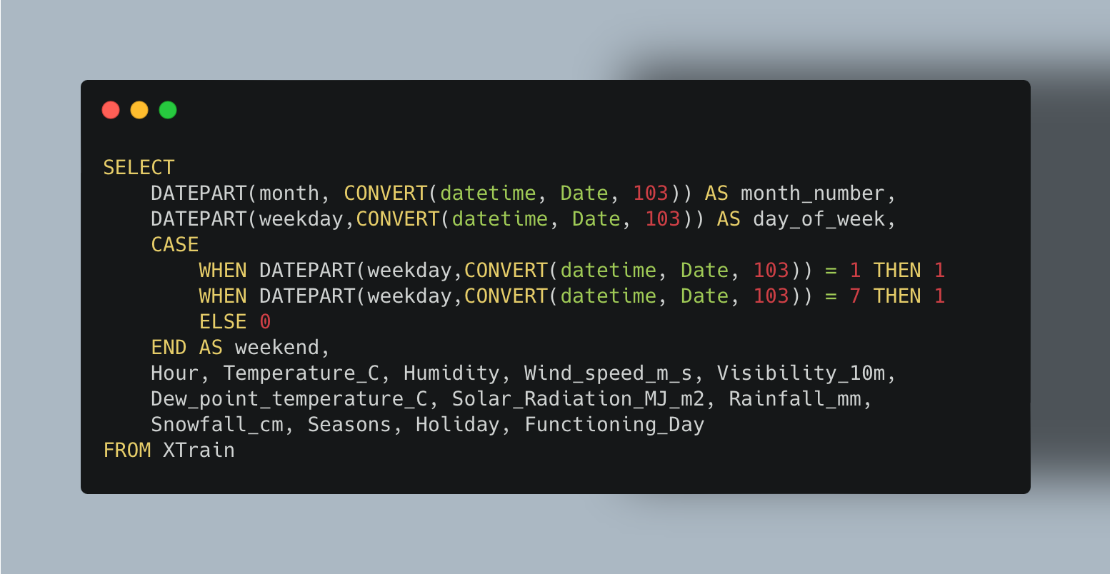
If you look at the XTrain data, you will see the data in the format that it was given. The date was given in the MM/DD/YYYY format. The following query was used to convert the column to the datetime format. The “103” key was used for this specific starting format. Furthermore, DATEPART was used to find out the specific day of the week and the month for each date. CASE was used to determine if that day was a weekend or not. These are all important features that can predict the number of bike rentals on a given day. Trivial features were excluded from the query.
The output of this query is shown below.
XTest can be queried in a similar fashion.
Using a SQL Query in Jupyter Notebook
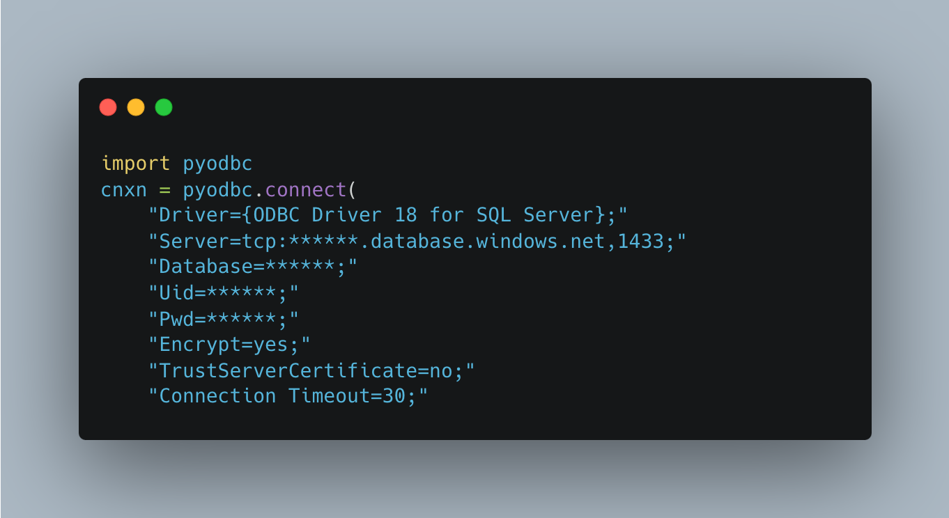
After the server was created in MS Azure, the following code was ran in Jupyter to connect the server. Of course, if you wish to replicate this, you will need to enter custom information about your server. Using MS Azure, this information can be found by clicking on your database and then clicking “connection strings” in the menu on the left.
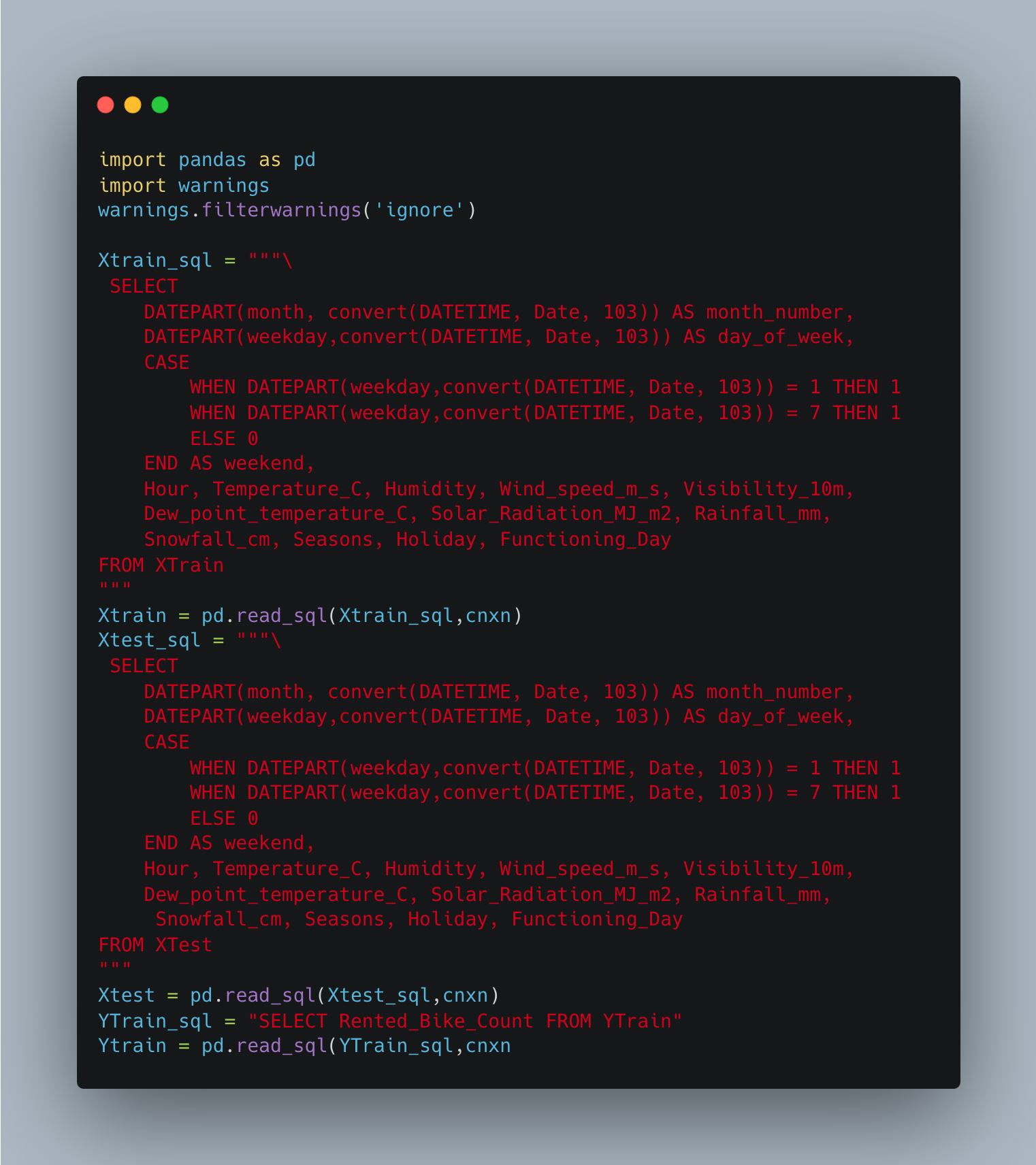
Next, the output of queries were converted into pandas dataframes. The queries for XTrain, XTest, and yTrain are shown below. As you can see, there is some code used to filter out a warning. This warning suggested using SQLAlchemy. However, using pyodbc didn’t cause any problems for me so I chose to ignore it.
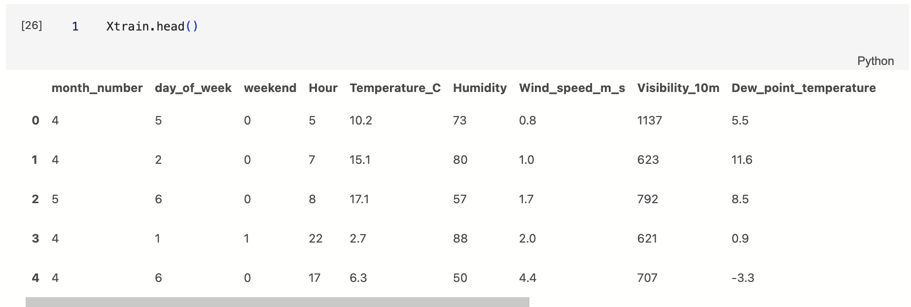
Printing Xtrain.head() in a new cell resulted in a dataframe that looked identical to the one queried earlier in SQL. This meant that my connection was succesful and I could move on to feature engineering and model building. How exciting!
One Hot Encoding
After my important features were selected, It was necessary to perform one hot encoding on the categorical data. One-hot encoding is a method used in machine learning to convert categorical data (like colors or types) into a numerical format that algorithms can understand. For each category, a new binary column is created, where “1” represents the presence of the category and “0” represents its absence. This transforms the categorical data into a machine-readable format without introducing an artificial order or importance among categories.
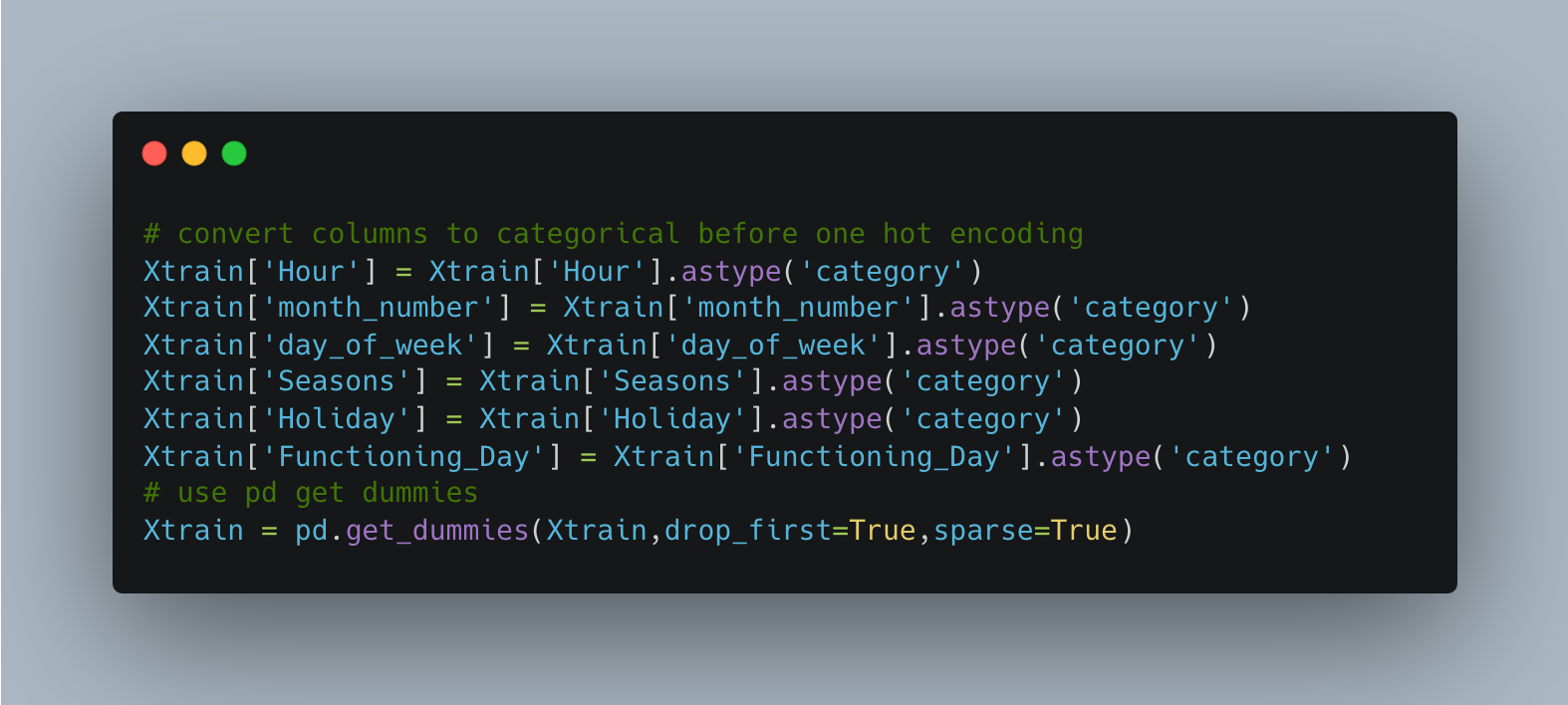
While one-hot-encoding can be done in SQL, pandas makes this relatively easy do do in Python. The columns that were to be one-hot-encoded were labeled as “category” type. Then the get dummies function was used to complete the process. The code to perform one-hot-encoding in Xtrain is shown below. This was also done for Xtest.
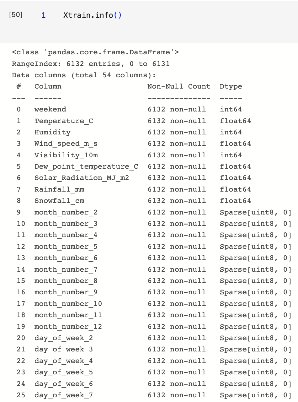
Running Xtrain.info() indicated that there were 54 columns. The image below shows how the “month” and “day_of_week” columns were one-hot-encoded.
Cross Validation
After one-hot-encoding, the training data was split into training and validation sets using sklearn. Since there was no yTest data given, it was necessary to split the training data into training and validation data. This way, the model could be built on the training data and tested for accuracy on the validation data. The code shown below was used to split the training data into 70% training data and 30% validation data.
Sizes of the Datasets:
- X train: (4292, 54)
- X val: (1840, 54)
- X test: (2628, 54)
- y train: (4292, 1)
- y val: (1840, 1)
Fixing the output distribution
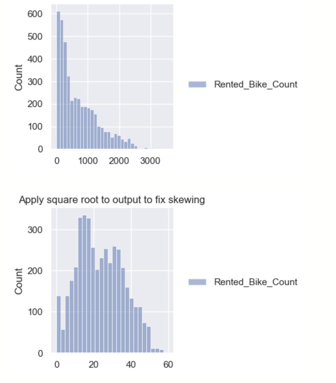
Machine learning models work much better when the output has a normal distribution. However, the output of X train was skewed right. In order to fix this, a square root was applied to the X train output. The distributions before applying the square root and after application are shown with Seaborn. This step should also be done with the validation data.
Training the Model
Several models were tried, but XGBoost yielded the highest R2 score on the validation data. The hyperparameters were also altered for optimal performance.
The R2 scores returned were:
- R2 on training: 0.9988912357447004
- R2 on validation: 0.9343343223928372
Unfortunately, the Kaggle competition is now closed and I can no longer retrieve the validation score for the test data. However, I remember it being very similar to the the validation data.
Here are some reasons XGBoost may be the most appropriate model for this dataset.
Robust Performance: XGBoost is known for its superior predictive accuracy, often outperforming other machine learning algorithms for structured or tabular data, such as the Seoul Bike Sharing Demand dataset. This has led to its dominance in applied machine learning and Kaggle competitions [2].
Ability to Handle Mixed Data Types: Your dataset contains a mix of categorical (like season, holiday, functional day) and numerical (like temperature, humidity, windspeed) features. XGBoost can effectively handle this mixture of feature types.
Handles Complex Non-linear Relationships: The relationship between features such as weather, time, and holiday status, and the demand for bikes is likely non-linear and involves complex interactions. XGBoost, being a gradient boosting algorithm, is capable of modeling these non-linearities and interactions effectively.
Overfitting Prevention: XGBoost includes built-in regularization parameters that help in preventing overfitting, making it a good choice for datasets with many features and complex relationships.
Handling Missing Values: If there are missing values in the dataset, XGBoost can automatically handle them.
Fast and Efficient: XGBoost is designed for speed and performance. It implements parallel processing, making it faster than many other ensemble classifiers. It also supports GPU training for further speed-up [1, 4].
Interpretability: Despite being a complex model, XGBoost provides feature importance scores which can be helpful for understanding the impact of different features on the predictions.
Key Findings
- The R2 score on the training data was about 0.9989.
- The R2 score on the validation data was about 0.9343.
What I Learned
- Most importantly, by re-visiting this project, I learned how to use SQL with Python using pyodbc.
- I learned how to set up a server on the MS Azure Portal.
- I learned the pros and cons of using different types of SQL.
- I learned how to use DATETIME and CONVERT in SQL.
- I used one-hot-encoding, normalized the output, and tested different machine learning models.
Conclusion
In conclusion, the project proved to be highly beneficial, particularly for a business involved in bike rentals. The primary objective was to achieve the highest possible R2 score on the test data, which was successfully attained. By using Python for data processing and model training and testing, in conjunction with SQL for data extraction and manipulation, an accurate predictive model was created.
This predictive model holds immense value for a bike rental business. With this, the business can anticipate the demand for rentals based on various factors. This level of foresight allows for better management of resources, reducing waste and saving costs. For example, knowing the demand in advance can help the business adjust the number of bikes needed at different times or locations, thereby avoiding unnecessary expenses related to bike maintenance or potential overstock.
Moreover, it can help with staffing decisions as personnel can be allocated according to anticipated demand. This further optimizes costs and improves customer service, as the business can ensure adequate staff is available when demand is high.
Ultimately, the individual successfully completed the project, achieving a high R2 score on the test data. The outcomes not only demonstrate the effectiveness of combining Python and SQL in predictive modeling but also highlight how data science can deliver tangible benefits to businesses by enabling them to make data-driven decisions, optimize their operations, and save money.
