Introduction
Iron ore, a vital ingredient for steel production, is extracted from minerals rich in iron oxides, displaying colors from dark grey to rusty red. Among these, high-grade ores with substantial hematite or magnetite content are particularly valuable. These ores, often surpassing 60% iron content, are directly used in steel-making processes.
However, the quality of iron ore isn’t solely determined by its iron content; impurities like silica play a crucial role. High silica levels can increase slag volume during smelting, affecting efficiency. Predicting silica content is essential for optimizing the manufacturing process and minimizing environmental impact.
This article delves into iron ore mining, highlighting the significance of monitoring silica concentration. By analyzing a specific dataset, the study uncovers patterns in the mining process and introduces a predictive model for iron and silica concentrate.
Dataset Overview:
- Origin: Real-world mining plants, focusing on a flotation plant.
- Purpose: Predict the amount of silica (impurity) in the ore concentrate in real-time.
- Time Frame: March 2017 to September 2017.
- Sampling: Data samples are taken every 20 seconds.
- Key Columns:
- Initial columns: Measures of iron feed and silica feed.
- Middle columns: Process data, including level and airflow in flotation columns.
- Final columns: Lab measurements of final iron ore pulp quality, with the last column indicating the percentage of silica. These columns serve as the output in the prediction model.
- Goal: Perform time-based analysis on the data to better understand it and to build a prediction model for impurity levels.
- Dataset Link: Quality Prediction in a Mining Process
This dataset provides insights into the mining process, aiming to enhance efficiency by predicting impurity levels in real-time and understanding patterns over time.
Time-Based Data Analysis
Data Loading and Preprocessing
The dataset, containing various parameters related to the mining process, was sourced from a CSV file. A key focus during preprocessing was the ‘date’ column, from which we derived multiple features such as the hour of the day, day of the week, month, and an indicator signifying weekends.
For this project, both SQL and Python were employed to handle and process the data. In a preceding endeavor—a bike rental prediction model—I utilized Azure to set up a database and conducted queries using T-SQL within Azure Data Studio. However, since my Azure subscription has since expired, I transitioned to SQLite for the current project. A significant advantage of SQLite is its ability to integrate seamlessly with Python, eliminating the need for external database hosting. On the flip side, SQLite lacks native Datetime functions.
Nevertheless, this limitation was circumvented by leveraging Python’s capabilities to perform Datetime operations. The initial step in preprocessing entailed transforming the Datetime information into a set of features that could be more efficiently interpreted by SQLite. Subsequently, SQLite was employed for conducting time-centric analyses.
Visualizations
Multiple visualizations were generated to understand the patterns in % Silica and % Iron concentrates based on different time granularities such as hour of the day and day of the week. The visuals provide insights into how the concentrations change over time. The visual below shows the average % Silica Concentrate per hour and the average % Iron Concentrate per hour for each time period. As you can see, the two concentrates tend to be negatively correlated.
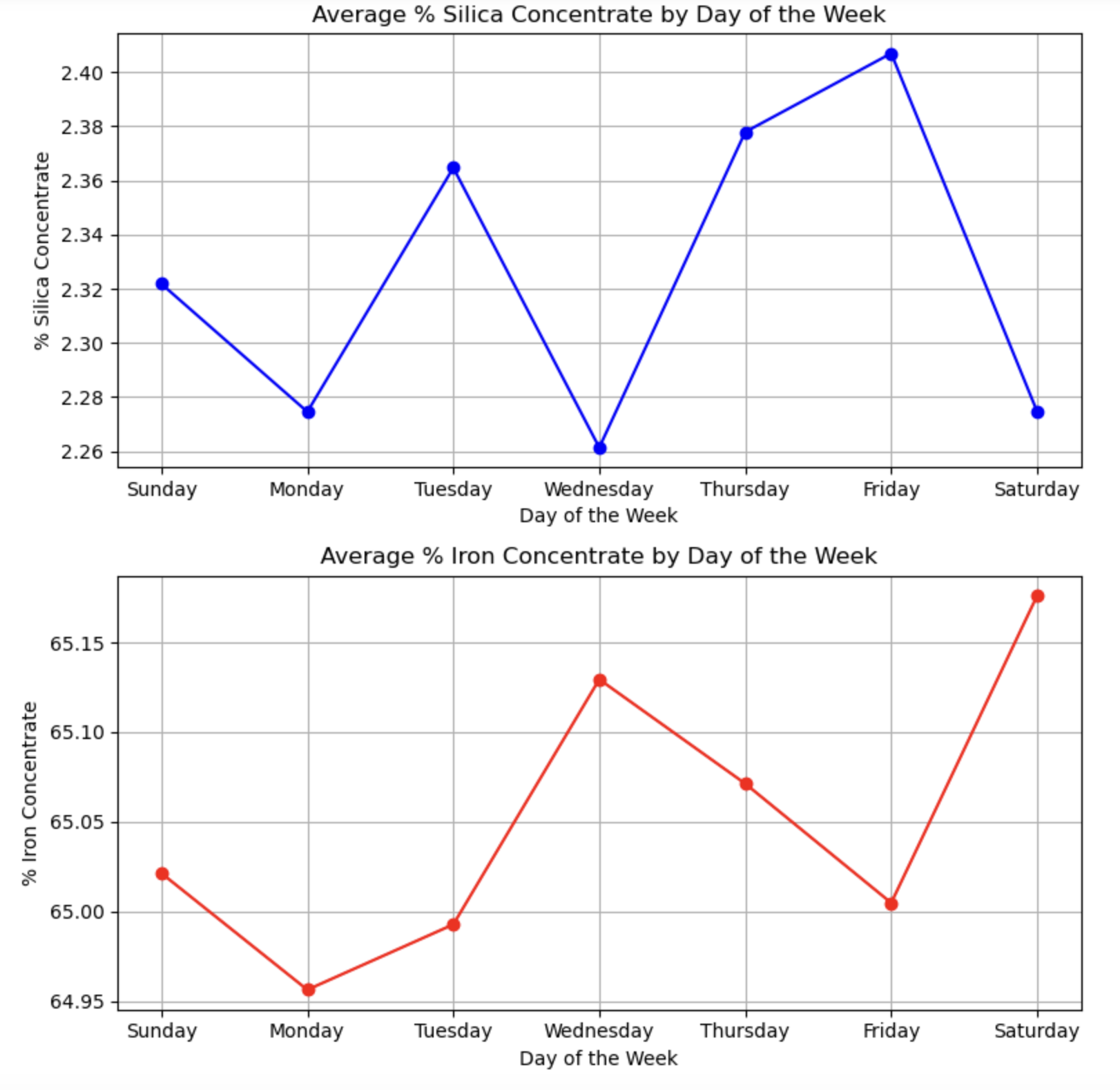
The chart provided illustrates the average percentage of Silica Concentrate for every day of the week. Once more, the graph underscores a negative correlation between the two Concentrates. Yet, Monday deviates from this observed trend. This suggests that while there’s a noticeable negative correlation, other factors certainly play a role and should be taken into account.
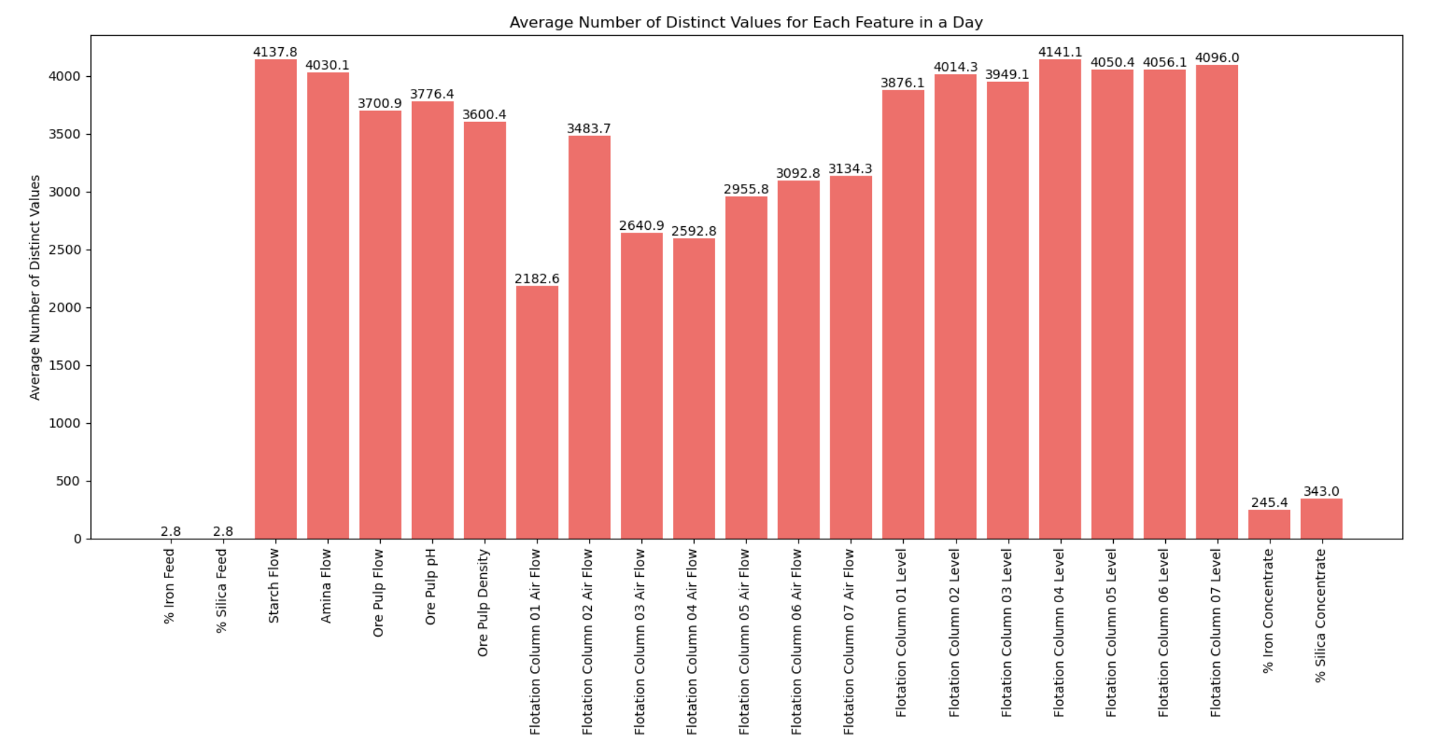
The following bar chart depicts the daily average of unique values for each feature. Notably, the iron and silicon feeds typically present fewer than 3 unique values each day. In contrast, some metrics, like starch flow, have an average of more than 4000 unique daily values. Given that the dataset records a sample every 20 seconds, this equates to 4320 samples daily. This information provides insight into the rate at which these values fluctuate throughout the day.
Predictive Modeling
Data Preparation - Contextual Variables
Data was split into features (X) and targets (y), where the targets are % Iron Concentrate and % Silica Concentrate. An 80-20 split was used to separate the data into training and test sets.
For our analysis, the dataset was divided into predictor variables (X) and response variables (y), where the response variables represent the % Iron Concentrate and % Silica Concentrate. We adopted an 80-20 split to segregate the dataset into training and test subsets.
In the process of preparing the data, it became necessary to critically evaluate the relevance of each feature. Drawing parallels from a prior bike rental demand prediction model I developed, factors like the day of the week and time of day played a significant role in forecasting demand. However, in the current context, such temporal variables seemed incongruous. To draw an analogy, the time taken for water to boil would ostensibly be the same on a Monday as it would on a Tuesday. If there were variations, they would likely be attributed to parameters such as the initial water temperature or the heat intensity of the stove, rather than the day itself.
Given this understanding, all features related to time and dates were prudently eliminated from our dataset. While this action might have led to a slight reduction in the R2 score, it ensures that our model is better tailored for predictions on future data sets. From a machine learning perspective, this step was crucial to prevent overfitting, ensuring that our model generalizes well to new, unseen data.
Data Preparation - Garbage in Garbage out
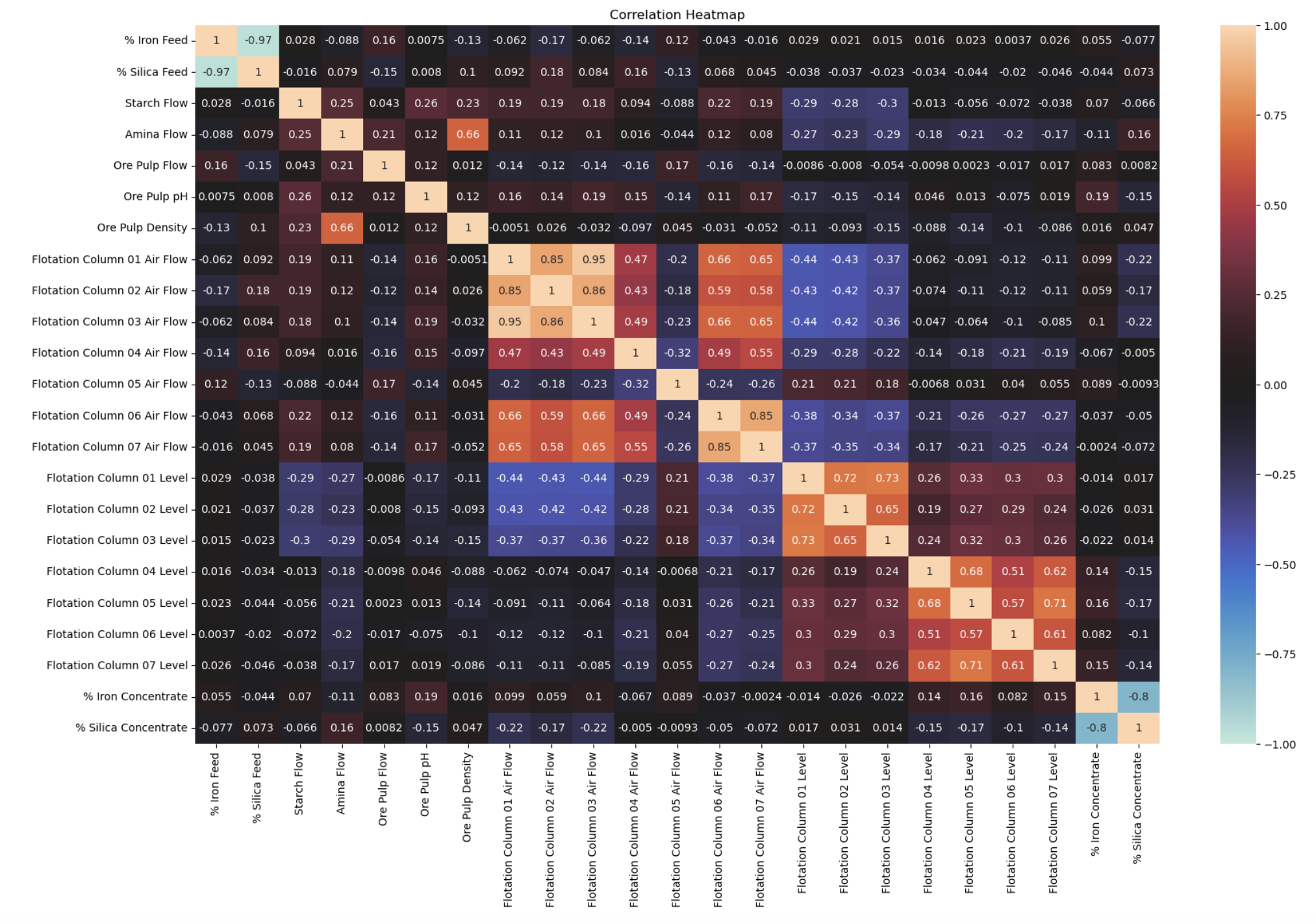
A heatmap was generated to visualize the correlation between variables. This visual representation aids in understanding the degree of association between different features.
There are two primary scenarios warranting the consideration of variable deletion:
High Inter-Variable Correlation: A classic instance of this was observed between “Flotation Column 01 Air Flow” and “Flotation Column 03 Air Flow”, which exhibited a correlation of 0.95. While some literature suggests removing variables with correlations exceeding 0.95, the research team decided to retain both columns. The correlation did not decisively surpass this threshold. Nonetheless, it might be valuable in future analyses to test the model’s performance by excluding one of these highly correlated variables.
Low Correlation with the Output: Variables that have minimal correlation with the target output might be considered for removal. However, in this study, even when some variables demonstrated very low correlation values (below 0.01) with one of the outputs, they did not consistently show low correlation across both target variables. Given the objective to craft a singular model addressing both outputs, the decision was made to retain all such variables. In the future, it may make sense to build seperate models for each output to achieve more accurate results.
Model Selection and Training
The data was split into 80% training and 20% testing data.
A RandomForestRegressor was chosen to predict the two targets. The model was trained on the training data to capture patterns in the input features that influence the concentrations. The number of iterations was set to 20.
Model Evaluation
The model’s predictions on the test set were evaluated using the Mean Squared Error (MSE) and ( R^2 ) score for both targets. These metrics provide a quantitative measure of the model’s accuracy and fit.
Random Forest Model Results
| Metric | Iron | Silica |
|---|---|---|
| MSE | 0.04238187206017949 | 0.04277235228583643 |
| R2 | 0.966036383564287 | 0.9661563706544567 |
Conclusion
In this study, time-based analysis was carried out using SQLite in Python. One of the advantages of using SQLite is that it doesn’t require setting up a separate database, making the process smoother and more efficient. With Python’s tools at hand, the analysis was straightforward and effective.
The data revealed changes in % Iron and % Silica concentrations over time, which is valuable information for those in the mining industry. A significant component of the research was the development of a machine learning model. This model is designed to predict concentrations based on certain features, providing a practical tool that could enhance efficiency in mining operations.
Overall, this project served as a solid learning experience in data science. By combining python with SQLite and using machine learning, it demonstrated the potential of data-driven decision-making.
In conclusion, the research highlighted the shifts in mineral concentrations over time and showcased the utility of tools like SQLite and machine learning in understanding and predicting such changes. It stands as a testament to the practical and educational value of hands-on data projects.


